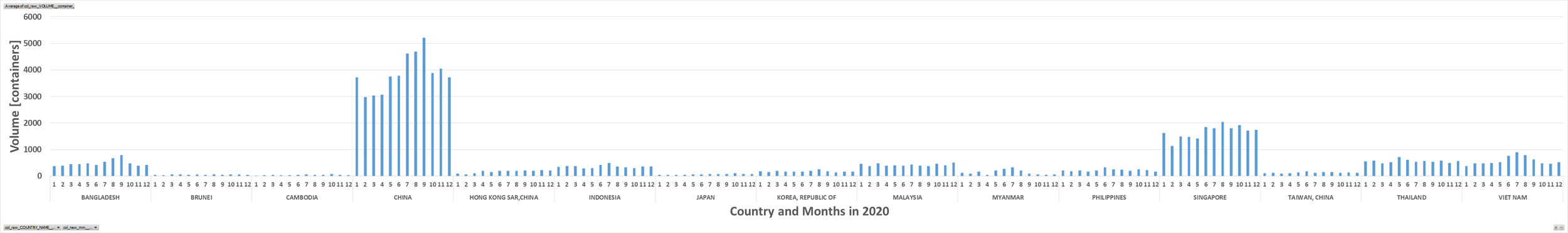
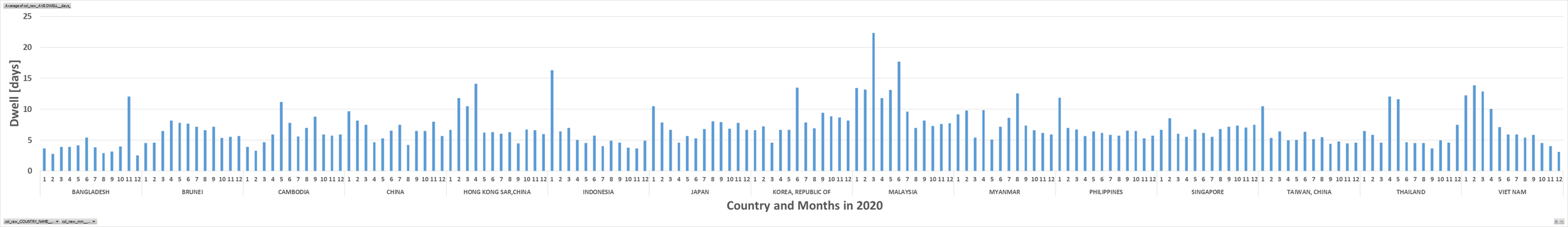
Data-Pivot-Chart

  
    Data-Pivot-Chart-Bar-Vertical
> y = Volume [containers]
> x = Countries (Asia), 2020.mm
  

  
    Data-Pivot-Chart-Bar-Vertical
> y = Dwell [days]
> x = Countries (Asia), 2020.mm
  

Data-Pivot-Chart

  
    Data-Pivot-Chart

Excel > Data Table 
> Select the whole table by
  > Ctrl + Home
  > Ctrl + Shift + Down + Right
> Insert > Charts > PivotChart > PivotChart & PivotTable
  > New Worksheet > OK

Pivot Table
> Populate
  > Drag drop categorical fields "Rows"
  > Drag drop numerical fields in "Values" section
> Format
  > Click into Pivot Table > Design
    > Subtotals     > Do Not Show Subtotals
    > Grand Totals  > Off for Rows and Columns
    > Report Layout > Show in Tabular Form
    > Report Layout > Repeat All Item Labels

Pivot Table Name
> Click into pivot table (any cell) 
  > Right-click > PivotTable Options
    > PivotTable Name

Slicer Connections and Settings
> Click into pivot table (any cell) 
  > Insert > Slicer
    > Right-click > Report Connections > Select Pivot Tables
    > Right-click > Slicer Settings > Hide items with no data
      
  

Contact